Insuring Against Going Viral: Life Expectancy on Spotify Top Charts

This project showcases a spectrum of technical skills in a nontraditional actuarial setting. Many methods are known for analyzing and predicting movement in a financial market and quantifying risk. We seek to give similar treatment in the case of Spotify's Top Charts, where popularity "drives up" the ranking (price) of a given index (song). In particular, we draw special attention to Queen's "Bohemian Rhapsody". Put concisely, in all of Spotify's public Top Charts history, until the release of the biopic film featuring Queen, the band has never placed in Spotify's Top 200 chart. Ever since the movie's release, even to this day, Queen has never failed to rank top 200 in the United States as well as globally. How long will this viral reign last? We investigate in a number of ways, ultimately estimating a total life of ~4 years on the US Spotify Top 200 Chart, and possibly more on Spotify's Global Top 200 Chart.

BACKGROUND

In recent years we’ve witnessed an emergence of music “biopics,” major films that follow the lives of musicians as they pave their way to success (i.e. Elton John's Rocketman (2019), The Beatles’ parody Yesterday (2019), Queen's Bohemian Rhapsody (2018), NWA's Straight out of Compton (2015), and many more). Surely a success story makes for a feel-good experience, and indeed, films like these educate millennials who might otherwise be blind to these artists. However, whether due to nostalgia or “double-dipping” success, these movies also serve a critical strategic purpose–they generate a lot of revenue.

The movie Bohemian Rhapsody alone generated $903.2 in box office sales, with much more revenue from sales of soundtracks, music streaming services, and live performance DVDs. It is important to note that a month before the movie’s release and prior, none of Queen's tracks was in any of Spotify’s historical top charts.

From Billboard Magazine:

"Queen earns its highest-charting album in 38 years, as the Bohemian Rhapsody film soundtrack surges 25-3 on the Billboard 200 with 59,000 units (up 187 percent) earned in the week ending Nov. 8 according to Nielsen Music, after the film’s opening in U.S. theaters on Nov. 2. Of its unit haul, album sales comprised 24,000 -- up 182 percent."

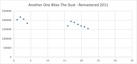
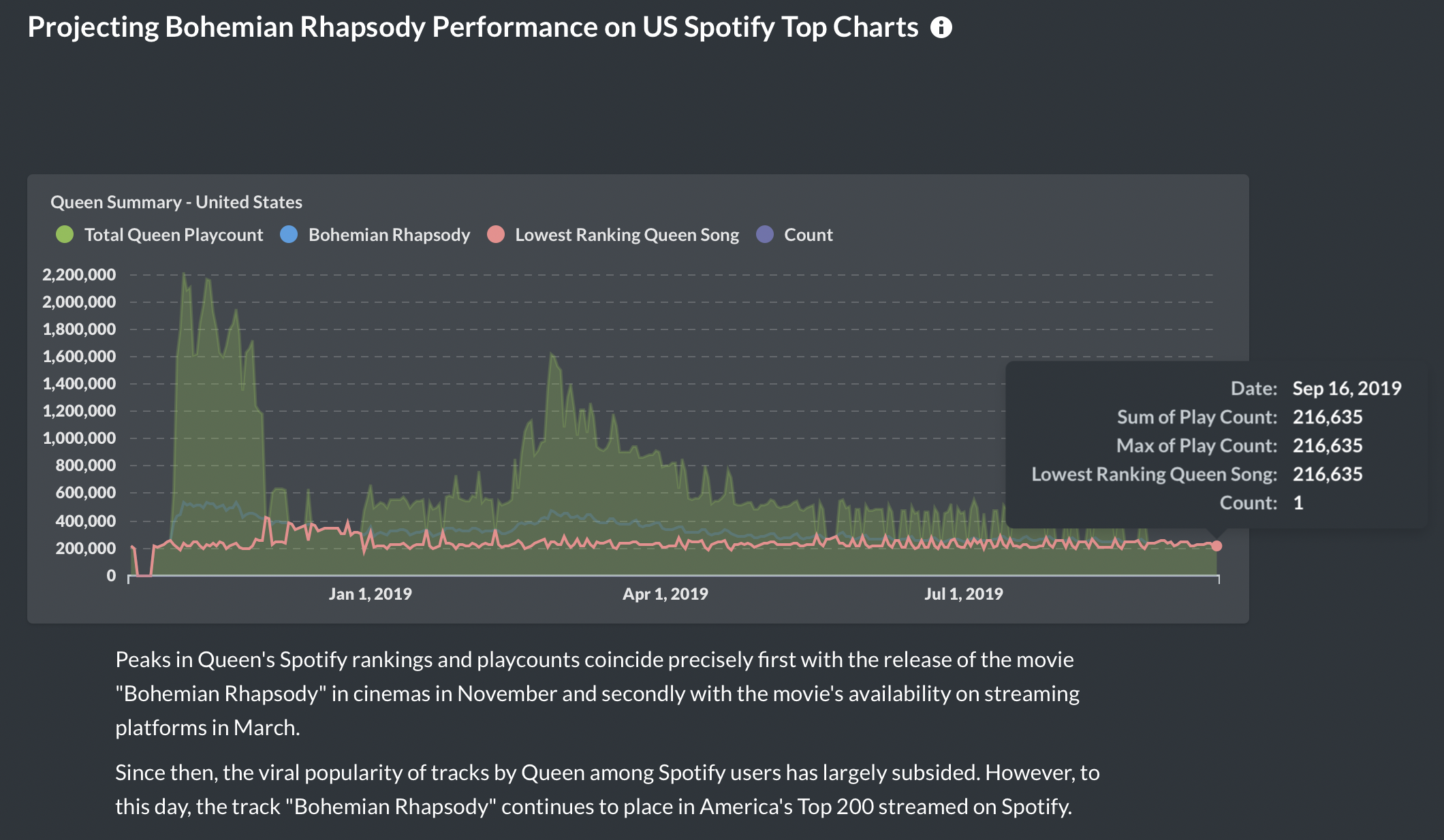
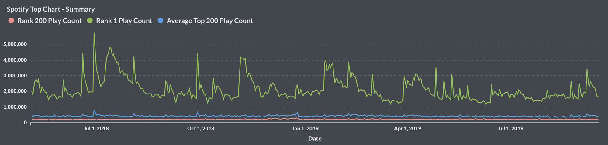
At the time of this study in Summer 2019, over 7 months after the movie's release, the track Bohemian Rhapsody is still consistently in the top 75 most-played in most regions, a feat near unimaginable for a song released so many years ago. Moreover, the song has since always been in the top 200 global charts, netting over 42 million stream plays a month globally on Spotify alone. One of our findings gives a highly conservative estimate that in a year, the single song "Bohemian Rhapsody" generates well over $10.7 million from Spotify streams alone.

The Relation to Insurance

Easily accessible and sharable content spreads with much less friction than does restricted content. This case study presents pricing  for music streaming services to reduce exposure to large losses due to royalty payments for viral content.

To maximize revenue and exposure, for most artists in the music industry, it is in their best interest to make their content accessible to a larger audience (and thus may accept lower per-play royalty for a greater volume of plays). For subscription-based music streaming services, to market consumers away from choosing competitors, the company must provide not only a vast selection of content but also the latest trending and viral content.

If a small or new streaming service pays flat royalty rates but only collects (monthly) subscription premiums, the company is exposed to potentially dangerous levels of loss in terms of paying royalties if provided content goes viral and invokes unexpectedly high play counts. Because offering the latest trending content does not guarantee a comparative advantage over competitors (who likely offer the same content), this increase in streaming of content is likely not met with an adequate increase in subscription premiums to offset loss from royalty payments.

Analyzing both direct and indirect effects of viral content, we propose an appropriate insurance product for small streaming services to address the above concerns.

---

About this Project

In this article, we first open with business intelligence approach, supposing that our only analytical tools are those from Microsoft Office products, namely Excel and Access. We use Excel's built in data scraping tools to experience its shortcomings. We generate dashboards in Excel with visualizations that can be used to support actuarial judgment and model assumptions. Generally, while this portion demonstrates the power of Excel, we also expose issues regarding lack of scalability.  

Next, we generalize to the use of more powerful and versatile programming tools, particularly PostgreSQL and R for everything from web scraping to analysis to data visualization.

---

PART 1 : Microsoft Office for Data Science: Web Scraping in Excel and Querying with Access

Navigating policy in the actuarial profession can be tricky. To meet regulatory restrictions set forth by the Actuarial Standards of Practice and government bodies, actuaries may face pressure to use outdated (and more commonly accepted) analyses techniques, such as iterated univariate rating models.

This presents an added difficulty to an actuarial problem at hand--using limited tools to perform a desired analysis. As a basic simulation of this, suppose we want to use only basis tools to dynamically track and analyze music artist performance on a streaming service like Spotify.  Particularly we are interested in the playcount distributions for tracks by that artist, and how that trends over time. Can we form predictions and forecasts for how we expect a track to perform?

In this project we'll follow Queen's performance on Spotify before and after the release of Bohemian Rhapsody, the major biopic following the story of Queen and lead singer Freddie Mercury (for the full project executed in R).

The Challenge:

Use ONLY Microsoft Office Suite. That's right, we're only allowed to use Excel, Word, and Access. Without more 'powerful' programming tools, what can we even do with Excel?

Turns out, quite a lot. Here's how:

Excel as a Data Scraping tool

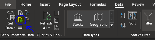
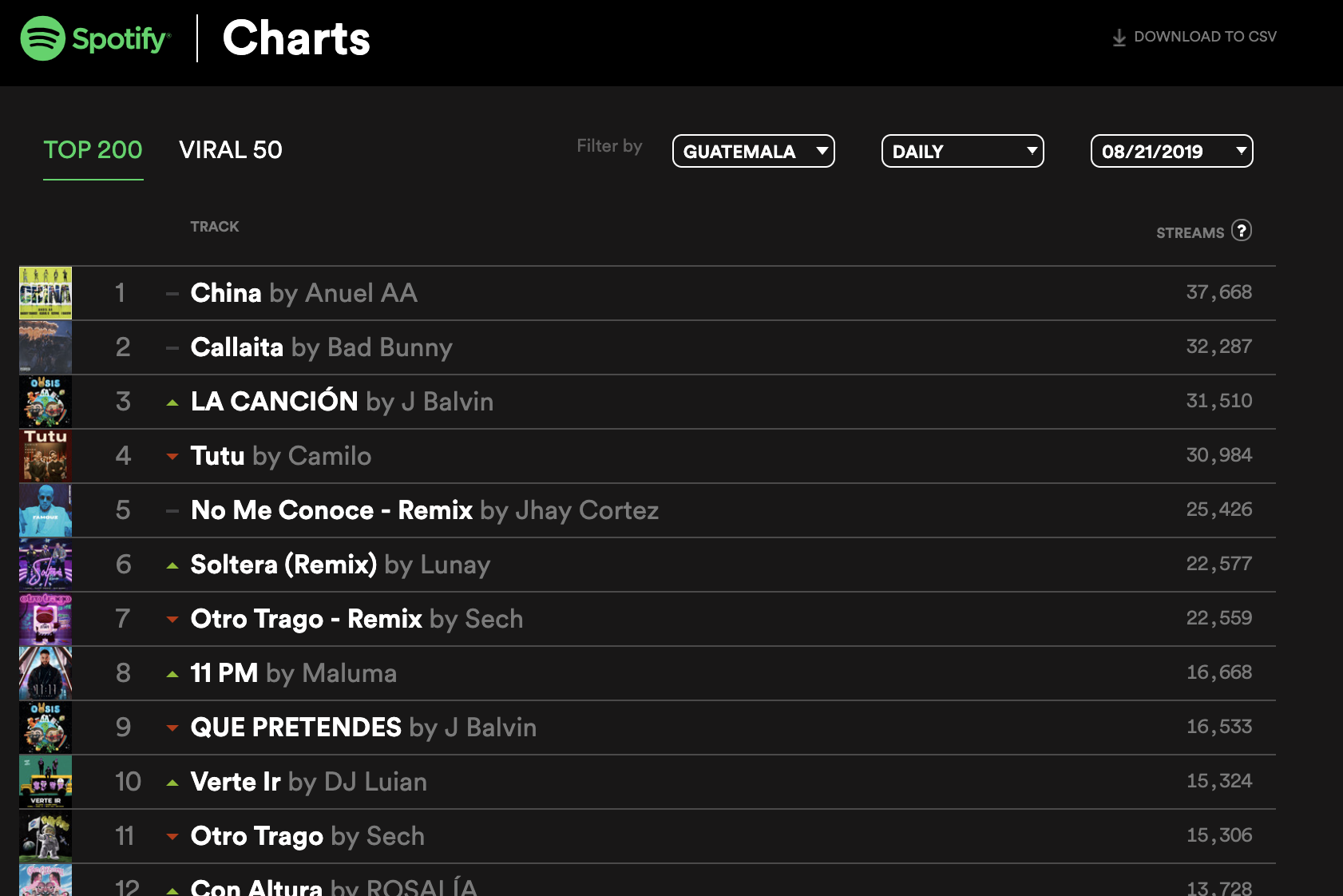
Spotify has an API that spoon feeds developers key metrics when requested via tools like Python and R, but if we're limited to Excel, we'll need to take a web-scraping approach. Excel has a built-in "get-data: external (from the web)" function, and Spotify provides pretty nice summary (Top 200) .csv's for each region, updated daily.

Using this tool, we can input any website url (https://example.com/website/path) and excel would scrape the page data into some sort of semi-coherent table. If our page actually has data tables, our output looks better. If our page is in .csv format, this Excel tool works just like downloading the .csv and manually loading it offline on our device.

We'll scrape data from https://spotifycharts.com. Surely we don't want to manually enter webpages for each day, and we don't want to use SpotifyChart's search function to scroll and click through each region and date. We want a smarter way to iterate through dates and pull the desired data.

We can do this in Excel.

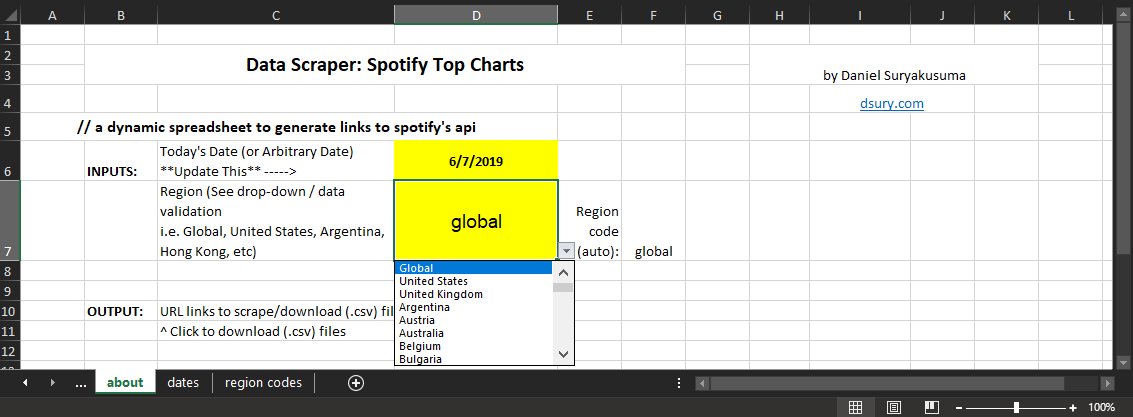
Spotify provides daily song ranking and playcount metrics for 64 regions. We create a drop-down menu on the main page for ease-of-use to perform an automated index-match for url generation.

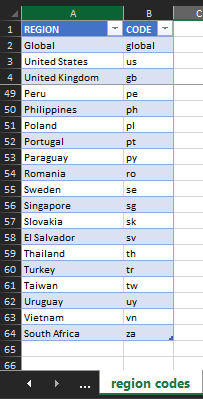
Using these region codes and today(), we can place some simple logic to automatically generate url's like the following:

https://spotifycharts.com/regional/global/weekly/2019-06-07--2019-06-14/download/
https://spotifycharts.com/regional/global/weekly/2019-05-31--2019-06-07/download/
https://spotifycharts.com/regional/global/weekly/2019-05-24--2019-05-31/download/
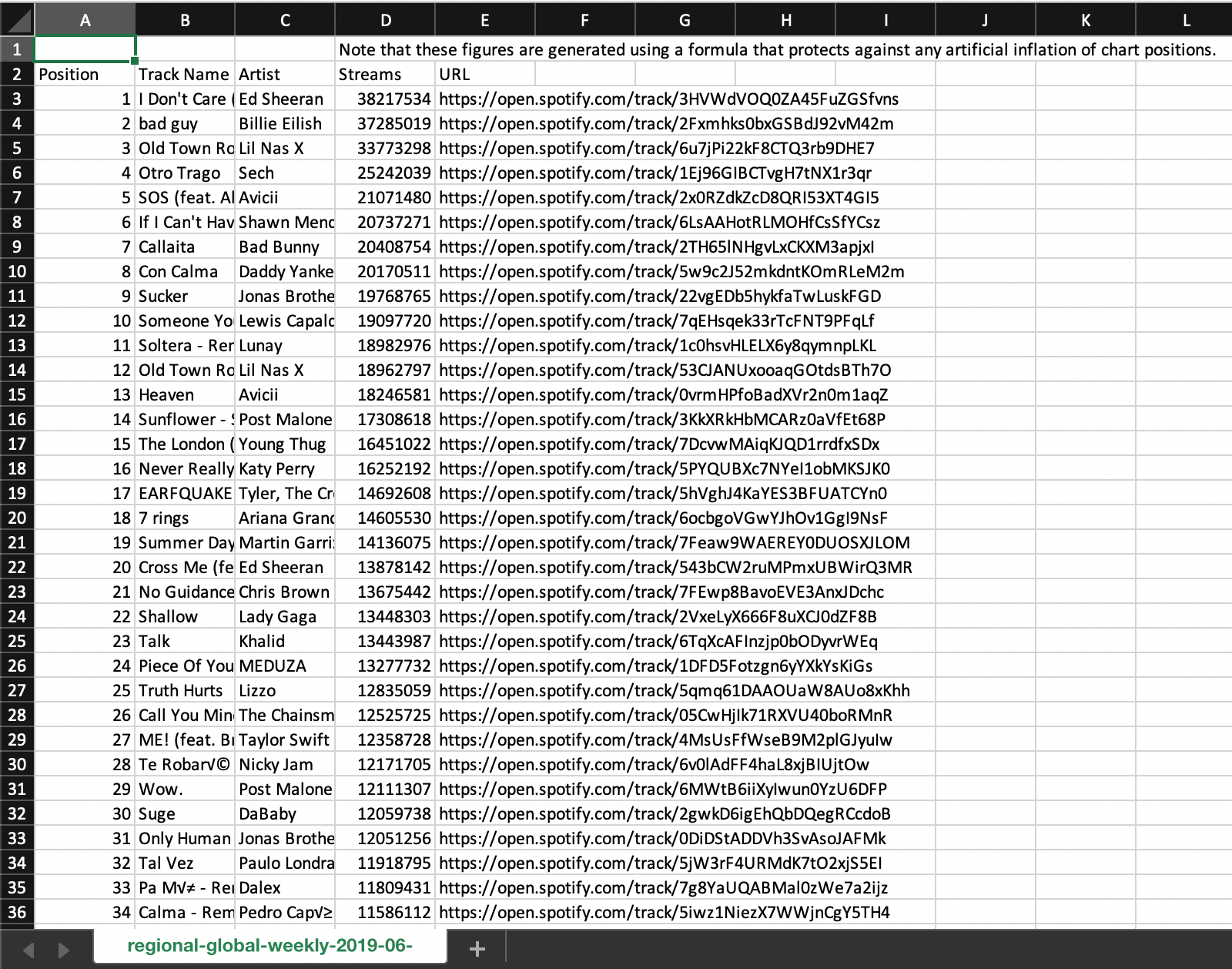
https://spotifycharts.com/regional/global/weekly/2019-05-17--2019-05-24/download/

Our spreadsheet looks like this:

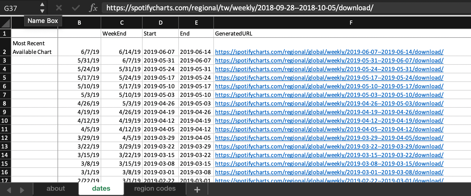
To generate our desired Spotify URLs:

#0. Get =today() 's date, and standardize to the most recent available weekly chart

=about!D6 - MOD(about!D6, 7) - 1

#1. Get date: start of week (Start column)

=TEXT(YEAR(B11),0)&"-" &IF( LEN(TEXT(MONTH(B11),0))<2, "0"&TEXT(MONTH(B11),0), TEXT(MONTH(B11),0))&"-" &IF( LEN(TEXT(DAY(B11),0))<2, "0"&TEXT(DAY(B11),0), TEXT(DAY(B11),0))

#2. Get date: end of week (End)

=TEXT(YEAR(C11),0)&"-" &IF( LEN(TEXT(MONTH(C11),0))<2, "0"&TEXT(MONTH(C11),0), TEXT(MONTH(C11),0))&"-" &IF( LEN(TEXT(DAY(C11),0))<2, "0"&TEXT(DAY(C11),0), TEXT(DAY(C11),0))

#3. Generate URL (GeneratedURL)

=HYPERLINK("https://spotifycharts.com/regional/"&about!$F$7&"/weekly/"&D11&"--"&E11&"/download/")

Now we have a text string column of URL's to .csv's of interest to feed into Excel's "get data" feature.

Data Storage

Because each weekly or daily "Top 200" chart is of the same size and has the same corresponding data type across different dates and regions, we can use a relational database (i.e. Microsoft Access).

Each .csv has content like this:

We'll want a VBA macro to select only the data we want (not the first two rows) and append them correctly.

1. Get the week's id (date) and append this to a column

Sub placeFirstDate()
'
' placeFirstDate Macro
'
' Keyboard Shortcut: Ctrl+j
'
    Selection.End(xlToLeft).Select
    Selection.End(xlUp).Select
    Selection.End(xlDown).Select
    Range("A202").Select
    Selection.PasteSpecial Paste:=xlPasteValues, Operation:=xlNone, SkipBlanks _
        :=False, Transpose:=False
End Sub
Sub extendDates()
'
' extendDates Macro
'
' Keyboard Shortcut: Ctrl+l
'
    Selection.End(xlToLeft).Select
    Selection.End(xlUp).Select
    Selection.End(xlToLeft).Select
    Selection.End(xlUp).Select
    Selection.End(xlToLeft).Select
    Selection.End(xlUp).Select
    Range("B1").Select
    Selection.End(xlDown).Select
    Range("A401").Select
    Range(Selection, Selection.End(xlUp)).Select
    Selection.FillDown
End Sub

2. Select and copy data of interest, and append to one single consolidated table (containing Spotify data for one region, across different dates).

This can be done in a variety of different ways. I took an inelegant solution of keyboard macro-ing.

The results look something like this:

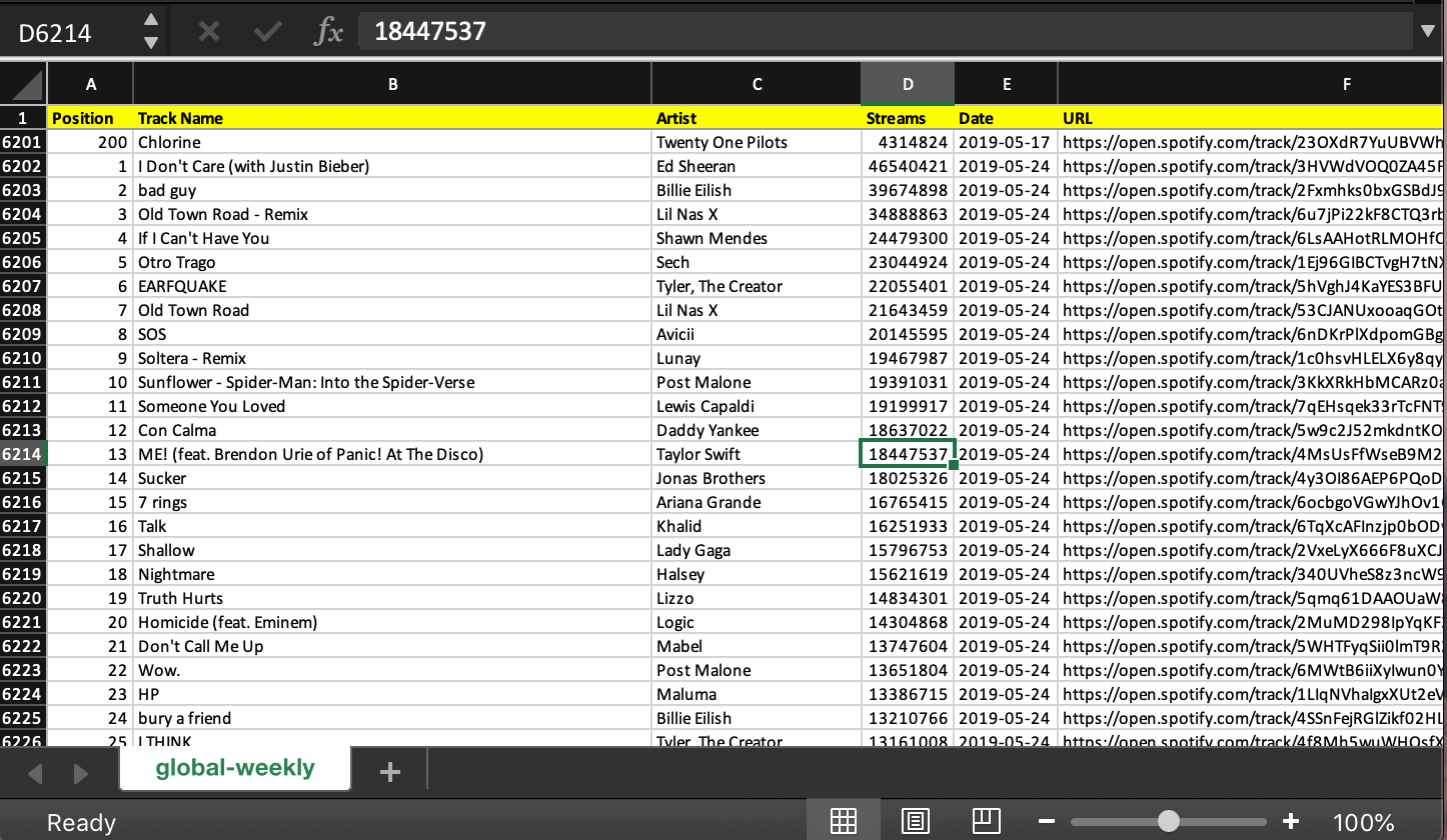
We could've cut and paste together these 7000+ rows of data by scrolling, clicking, downloading each .csv from SpotifyChart's data, but the key point here is the reproducibility and error prevention of our automated approach.

We can perform our analyses purely in Excel, but we opt for more power via SQL and Access.

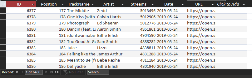
Querying Our Data:

Now we can import our data into Microsoft Access and perform queries (and queries on queries) to help with our analyses.

Now we're ready (and excited to) perform some queries:

Get entries of "Bohemian Rhapsody" only:

SELECT tblReference.Date, tblReference.Streams
FROM tblReference
WHERE (((tblReference.TrackName) Like "*bohemian*"))
GROUP BY tblReference.Date, tblReference.Streams;

Get the playcount of the #200 song on the chart (all songs with lower playcount did not make the list):

SELECT tblReference.Date, Min(tblReference.Streams) AS MinOfStreams
FROM tblReference
GROUP BY tblReference.Date;

Get the total playcount of ALL Top 200 songs during given time period:

SELECT tblReference.Date, Sum(tblReference.Streams) AS SumOfStreams
FROM tblReference
GROUP BY tblReference.Date;

Get the total playcount of all Queen tracks during the time period:

SELECT tblReference.Date, Sum(tblReference.Streams) AS SumOfStreams
FROM tblReference
WHERE (((tblReference.Artist) Like "*Queen*"))
GROUP BY tblReference.Date;

Get an entire summary table (getSummaryTable; Now a more complicated query off queries):

SELECT tblreference.date, 
       tblreference.trackname, 
       tblreference.streams, 
       [tblreference] ! [streams] / [getbohemianonly] ! [streams]             AS
       Ratio_to_BH, 
       [tblreference] ! [streams] / [getmin200] ! [minofstreams]              AS
       Ratio_to_rank200, 
       [tblreference] ! [streams] / [getglobalsum_queenonly] ! [sumofstreams] AS
       Perc_of_Queen, 
       [tblreference] ! [streams] / [getglobalsum] ! [sumofstreams]           AS
       Perc_of_All 
INTO   tblsummary 
FROM   (((tblreference 
          LEFT JOIN getglobalsum 
                 ON tblreference.date = getglobalsum.date) 
         LEFT JOIN getglobalsum_queenonly 
                ON tblreference.date = getglobalsum_queenonly.date) 
        LEFT JOIN getmin200 
               ON tblreference.date = getmin200.date) 
       LEFT JOIN getbohemianonly 
              ON tblreference.date = getbohemianonly.date 
WHERE  (( ( tblreference.artist ) LIKE "*queen*" )) 
GROUP  BY tblreference.date, 
          tblreference.trackname, 
          tblreference.streams, 
          getbohemianonly.streams, 
          getmin200.minofstreams, 
          getglobalsum_queenonly.sumofstreams, 
          getglobalsum.sumofstreams, 
          [tblreference] ! [streams] / [getbohemianonly] ! [streams],
          [tblreference] ! [streams] / [getmin200] ! [minofstreams], 
          [tblreference] ! [streams] / [getglobalsum_queenonly] ! [sumofstreams]
, 
          [tblreference] ! [streams] / [getglobalsum] ! [sumofstreams]; 

Visually, these queries in Access look like:

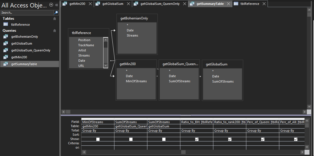
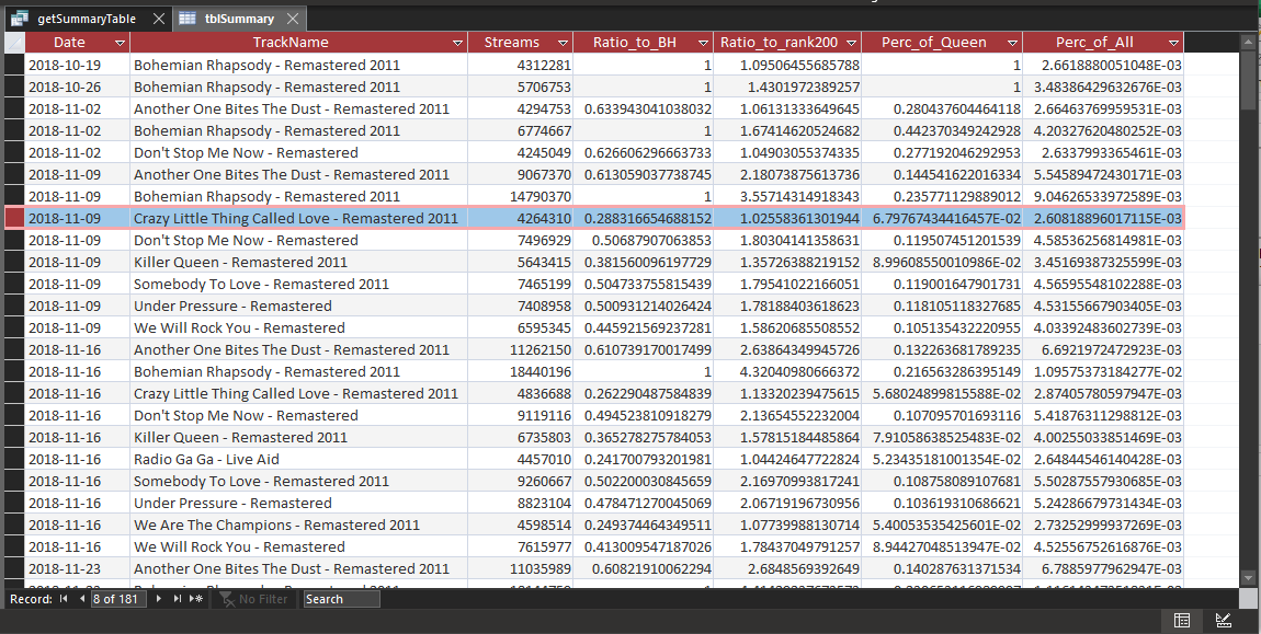
Now from our summary table, we have the following columns of data (above):

• Total Queen Streams (for the week)
• Total Top 200 Streams (for the week)
• Ratio of playcount to that week's #200
• Ratio of playcount to "Bohemian Rhapsody"

With our Access database, we can pull a PivotChart report:

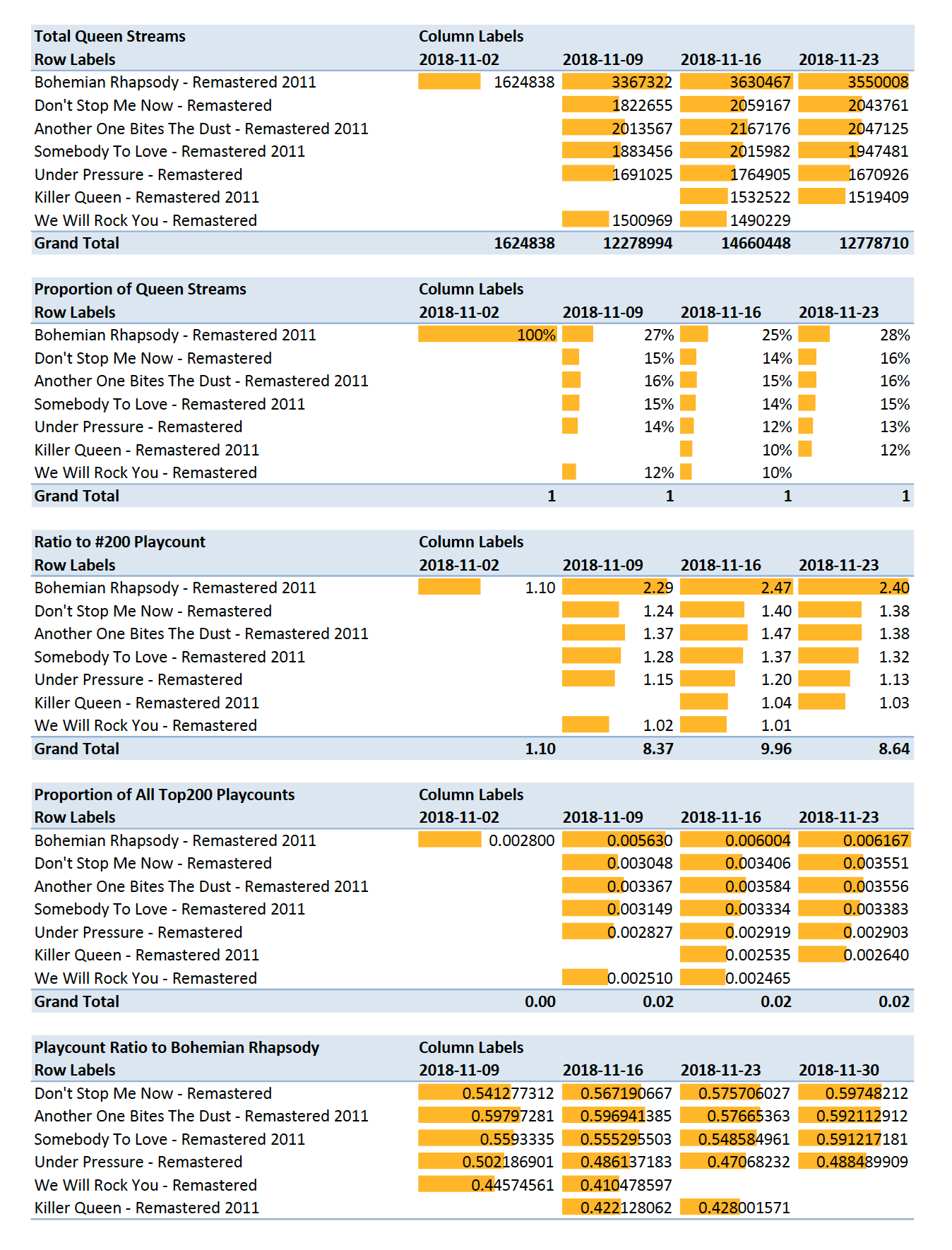
Dashboarding

The conditional formatting: data bars help us see a bit of the trends, but let's make responsive dashboards that adapt to new data inputs.

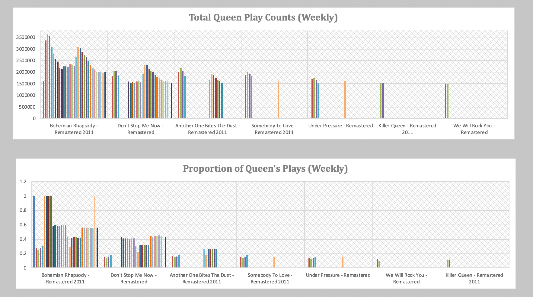
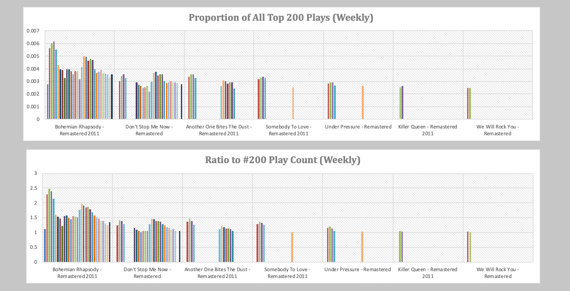
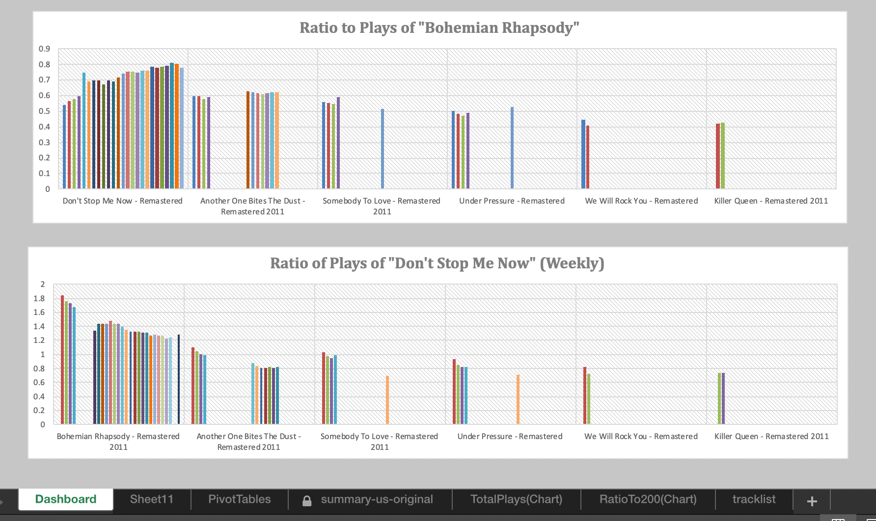
With this dashboard, we can gain a lot of intuition behind the data driving these plots. We can try models and see how they perform over time.

For a more in-depth analysis of this data set and prompt, we generalize in the next section to using R and PostgreSQL to estimate royalty costs for viral content.

---

PART 2 : Web Scraping in R: Scalability and Automation

Companies often make APIs available (application programming interfaces) to help developers make use of data to create neat apps. One popular example is Spotify, which makes much of its Web API data available for developers free of charge.

However, suppose we want to generate a report on a dataset that is not readily available (actuaries often encounter this problem with CY, AY, PY aggregation, where readily available data may not give the best granularity or result, but sometimes actuarial judgment must be exercised to acknowledge when data sets are sufficient to generate 'good enough' results). For large data sets, we need some way to 'clean' and prepare the data for analysis--compiling data into some database where we can query data, perform analyses, and generate reports.

Spotify does half the work for us, providing the actual Top Charts rankings with stream playcounts. True web scraping requires only minor adjustments in extracting useful data amidst noisy web channels. Our problem is that downloading each of these and using Excel+VBA to stitch them together requires too much human oversight and keypresses (time and energy), so we automate this process with data frames in R with a single function call.

Spotify generously presents us with a perfect opportunity to test this process, as its API and public charts permit developer access (and generally responds well to incessant pings requesting data). We kindly target https://spotifycharts.com to scrape and compile our desired data. In a past article, we used MS Excel's 'Get Data' function to scrape web data off the web page, and we used VB macros to 'intelligently' compile dozens of .csv datasets into a consolidated large database. However, this process scales poorly for larger datasets. Our interest is automating this process, with the following design goal in mind.

Goal: Minimize actions required by the user. A user should be able to simply specify "n" (days or weeks) duration and download a computer-generated compiled list of playcounts and rankings for a specified "region" (or all available regions).

Motivation for Scalability:

We can scrape .csv's for each day and week's Top 200 chart per region as made available by SpotifyCharts.com; however, this is far from sufficient for one attempting time-series data analyses or comparisons across regions. For example, to do so using our old procedure, we would have to manually stitch together 31 separate csv's, employing VBA macros to attaching fields indicating to which date these 200 rows of data correspond when compiled into one large list. Moreover, if we want to compare two regions over one month, this requires 31 x 2 separate csv's, and so on.  If we have any hopes of our project scaling to larger implications, we need a more intelligent way of meeting this demand than excel-macro bashing.

Creating a Web-Scraper From Scratch:

Before performing actuarial or statistical analyses on our data, we of course need to compile our necessary data. We choose R over Python, although both possess great libraries and tools. Obviously many web-scraping tools are available and open-source, but our desire is to develop our own data-scraper from scratch. We only truly use R's built-in read.csv and write.csv functions. For convenience, we use:

library('lubridate') # handles dates nicely for actuarial purposes
# library('mondate') # can be helpful but not used
# library('readxl') # can be helpful but not used
library('httr') # used to ping if a url exists, else don't scrape a page that doesn't exist

First we want to generate the correct dates to query/webscrape from Spotify. We'll start with weekly data then generalize to scraping daily charts.

# weekly
getWeeklyDates <- function(n = 52) {
  # n : number of weeks (defaults to 1 year)
  td <- Sys.Date() # today's date
  offset.date <- as.numeric( td - as.Date("2018-11-02") ) %% 7 # gets latest previous friday
  latest.available <- td - offset.date

  end.dates <- rep(latest.available, n) - 7 * seq(0,n-1,by=1) 
  # start.dates.vec <- 
  start.dates <- c(tail(end.dates, n - 1), tail(end.dates,1) - 7)
  dates <- data.frame(start = as.Date(start.dates), end = as.Date(end.dates))
  return(dates)
}


getWeeklyURL <- function(n = 52, region='global') {
  # region : region code (i.e. us, hk, gb)
  #   to-do : shiny dropdown for region selection
  # n : number of weeks
  
  x <- getWeeklyDates(n)
  a <- x$start 
  b <- x$end
  
  base0 <- 'https://spotifycharts.com/regional/'
  # region here
  base1 <- '/weekly/'
  # date$start here 
  base2 <- '--'
  # date$end here
  base3 <- '/download/'
  
  url.vec <- c()
  for (i in 1:n) {
    new.url <- toString(paste0( base0, region, base1, a[i], base2, b[i], base3, sep = ""))
    url.vec <- c(url.vec, new.url)
  }
  return(url.vec)
}

These above give us the correct dates to query from SpotifyCharts (which theoretically should not return errors when scraping). Confident, we perform the read/write of csv's:

# function to intake n

getSpotifyWeekly <- function( n=1, region='global' ) {
  # n : number of weeks (default 1 week)
  # region : (i.e. 'global', 'us', 'gb', ...)
  
  # vectors into df
  rankings <- matrix(data=NA, nrow = n*200, ncol = 1)
  songs <- matrix(data=NA, nrow = n*200, ncol = 1)
  artists <- matrix(data=NA, nrow = n*200, ncol = 1)
  playcounts <- matrix(data=NA, nrow = n*200, ncol = 1)
  dates <- matrix(data=NA, nrow = n*200, ncol = 1)
  urls <- matrix(data=NA, nrow = n*200, ncol = 1)

  # add date reference for comparing/combining dfs
  weeks <- getWeeklyDates(n)
    
  # list of csv's
  url.vec <- getWeeklyURL(n, region)
  
  # one week's csv at a time
  for (i in 1:n) {
    csv <- read.csv(file = url.vec[i], skip=1, header = TRUE)

    idx <- (i-1)*200 + 1
    idxs <- idx:(idx+199)
    dates[idxs] <- matrix(data=toString(as.Date(weeks$end[i])), ncol = 1)
    rankings[idxs] <- matrix(data = csv$Position, ncol = 1)
    songs[idxs] <- matrix(data = csv$Track.Name, ncol = 1)
    artists[idxs] <- matrix( data = csv$Artist, ncol = 1)
    playcounts[idxs] <- matrix( data = csv$Streams, ncol = 1)
    urls[idxs] <-matrix( data = csv$URL, ncol = 1)
    
    print(i); print(region); # debugging
  }
  
  # compile 
  spotify.data <- data.frame(dates = dates, rankings = rankings, songs = songs, artists = artists, playcounts = playcounts)
  
  #write into csv
  write.csv(spotify.data, file=paste0('spotify-',region,'-',Sys.Date(),'-export-',n,'-weeks.csv'))
}

Now we have everything we need to write large files with one line of code:

getSpotifyWeekly()

Now if we want different regions and to specify a time-span (default is 52 weeks = 1 year) backwards from today, we use:

for (rgn in regions) {
           getSpotifyWeekly(n=52, region = rgn)
}

where we perform a once-in-a-lifetime specification across all regions tracked and made publicly available by Spotify:

regions <- c('global','us','gb','ar','at','au','be','bg','bo','br','ca','ch','cl','co','cr','cz','de','dk','do','ec','ee','es','fi','fr','gr','gt','hk','hn','hu','id','ie','il',
'in', # india has 2/28/2019 earliest available
'is','it','jp','lt','lu','lv','mt','mx','my','ni','nl','no','nz','pa','pe','ph','pl','pt','py','ro','se','sg','sk','sv','th','tr','tw','uy','vn','za')

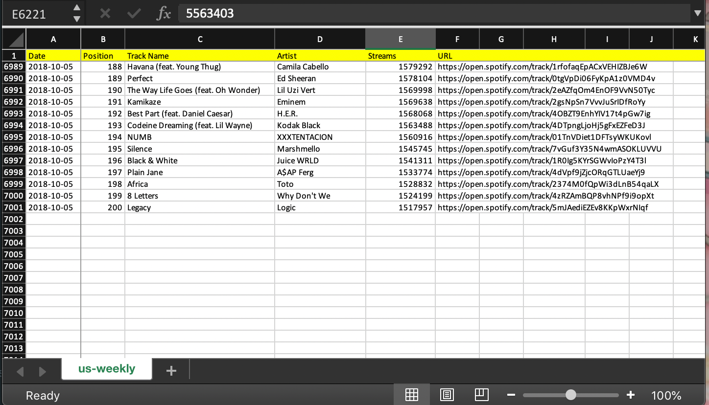
and that's all! We successfully stitched together 52 .csv's, appropriately managing data frames and adding a field to label a particular Top 200 chart to the date to which it corresponds. Here's a sample:

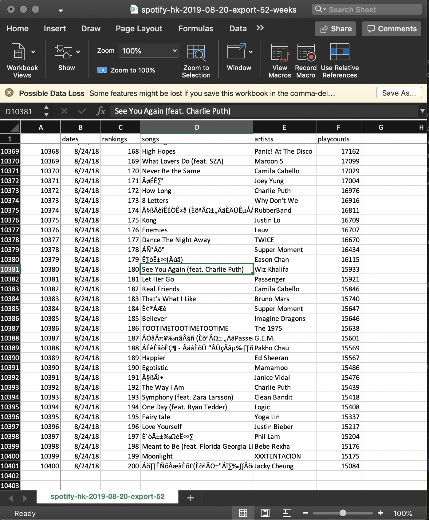
Wiz Khalifa's "See You Again" is still making the Top 200 chart? We could ask a lot of interesting questions about these anomalies. In particular, we'll be looking at Queen's "Bohemian Rhapsody".

Notice the 'loss' of foreign character accuracy when stored as .csv. If we write into .xlsx, we can get song and artist names in the correct characters; however, assuming we are interested in performing analyses on English titles, we keep it this way in the interest of smaller filesize (comma-delimited, .csv).

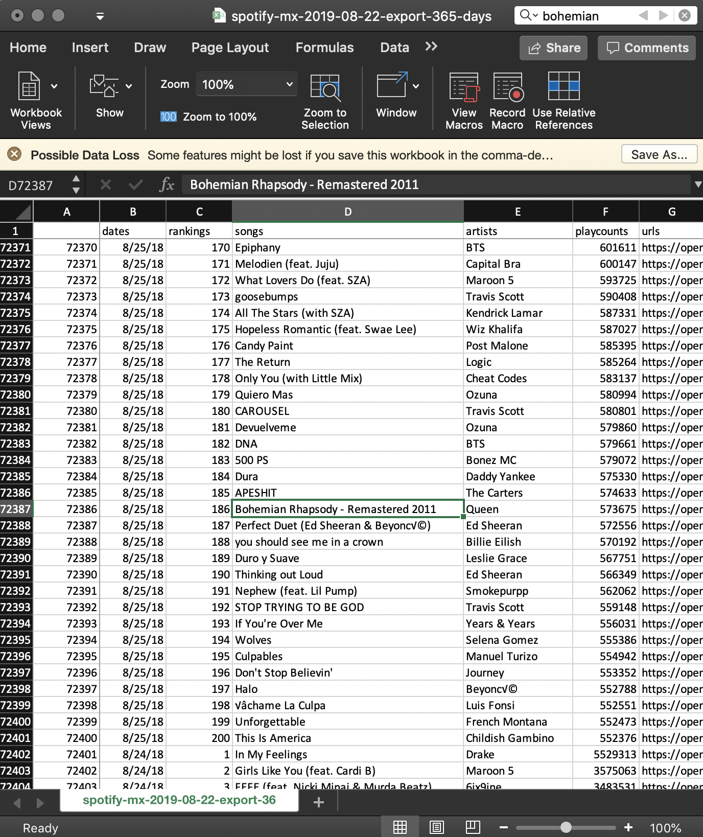
Spotify Daily Charts

Now we generalize to Daily Top 200 Spotify Charts. To review a region's chart over one year requires stitching together 365 .csv files, with 73,000 lines of data. If we want to look at more than one year (say 3), and compare 5 regions (out of 63 available on SpotifyCharts), this explodes to 5475 .csv files for a total of 1,095,000 lines of data. The benefit from scalability of our web scraping process is immediately evident.

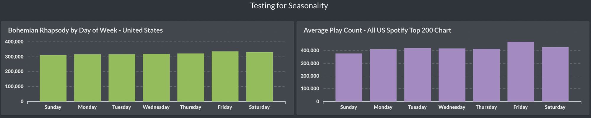
For further motivation, suppose we want to analyze seasonality of artists or songs, such as if a particular track gets more plays on the weekend versus weekdays. Or similarly, we may expect Holiday tracks to have higher playcounts near December, but perhaps we're interested in quantitating this with finer granularity.

- Is it actually true that people start listening to Christmas music right after Halloween?
- Precisely when do people stop listening to Holiday music?
- How does this sort of phenomenon vary around the world?

Generalizing to Daily Top Charts is simple (we don't have to standardize to Spotify's available weekly schedule), but we add precautions in case a particular day's data is unavailable (an error halts the entire procedure).

# library(httr) # need this for http_error() check

getDailyDates <- function(n = 365) {
  # n : number of dates
  # returns a vector of dates to scrape from spotify
  yd <- Sys.Date() - 1 # yesterday
  return( as.Date(rep(yd, n) - seq(0,n-1,by=1)) )
}

# generate matrix of urls
getDailyURL <- function(n=365, region='global') {
  x <- getDailyDates(n)
  
  base0 <- 'https://spotifycharts.com/regional/'
  # region here
  base1 <- '/daily/'
  # date here
  base2 <- '/download/'
  
  urls <- matrix(data = NA, ncol = 1, nrow = n)
  for (i in 1:n) {
    urls[i] <- paste0(base0, region, base1, toString(x[i]), base2)
  }
  return(urls)
}

## Compile data into one .csv
getSpotifyDaily <- function(n=365, region='global') {
  days <- getDailyDates(n)
  scrapes <- getDailyURL(n, region)
  
  rankings <- matrix(data=NA, nrow = n*200, ncol = 1)
  songs <- matrix(data=NA, nrow = n*200, ncol = 1)
  artists <- matrix(data=NA, nrow = n*200, ncol = 1)
  playcounts <- matrix(data=NA, nrow = n*200, ncol = 1)
  dates <- matrix(data=NA, nrow = n*200, ncol = 1)
  urls <- matrix(data=NA, nrow = n*200, ncol = 1) # listen on spotify
  
  for ( i in 1:n ) {
    curr.url <- scrapes[i]
    idx <- (i-1)*200 + 1
    idxs <- idx:(idx+199)    
    
    if (! http_error(curr.url) ) {
      csv <- read.csv( curr.url, header=TRUE, skip=1 )

      dates[idxs] <- matrix(data=toString(as.Date(days[i])), nrow = 200, ncol = 1)
      rankings[idxs] <- matrix(data = csv$Position, nrow = 200, ncol = 1)
      songs[idxs] <- matrix(data = csv$Track.Name, nrow = 200, ncol = 1)
      artists[idxs] <- matrix( data = csv$Artist, nrow = 200, ncol = 1)
      playcounts[idxs] <- matrix( data = csv$Streams, nrow = 200, ncol = 1)
      urls[idxs] <-matrix( data = csv$URL, ncol = 1)
      
      print('success') # debugging
    } # else leave as NA and move on
    
    print(paste(i,'days in',region))
  }
  
  # compile 
  spotify.data <- data.frame(dates = dates, rankings = rankings, songs = songs, artists = artists, playcounts = playcounts, urls = urls)
  
  # write into csv
  write.csv(spotify.data,file=paste0('spotify-',region,'-',Sys.Date(),'-export-',n,'-days.csv'))
  
}

and using the same 'regions' variable, we're now ready for:

for (rgn in regions) {
	getSpotifyDaily(n = 365, region = rgn)
}

Conclusion

With these, we have successfully performed our data scraping, with heaps of Spotify Charts data at our disposal for offline access. If we require data for a larger time period or desire more recent (realtime) data, it's only a single function call away.

getSpotifyDaily(n,region)

We now have everything we need to proceed with offline data analysis.

At the time of this article (8/22/2019), 1-year historical data (aggregated daily and weekly) is available hosted on this website. Full credits and thanks go to Spotify for making this data available publicly for scraping.

---

PART 3 : Statistical Analysis and Modeling in R

The analysis and automation in this section is done in R and Postgres, integrating into a live real-time dashboard.

An offline version of the dashboard and database snapshots (.sql, .csv, .json) are available at my Github.

When time permits, I will upload a full walkthrough here.

---

Future Direction of this Project

I am currently working on automating the workflow to update results on a daily basis and send summaries via email or Slack notification. This would be akin to a deliverable software product for a content streaming service client to monitor risk exposure due to trending and viral songs.