I recently had the opportunity to participate in UC Berkeley's Actuarial case competition, hosted by the Cal Actuarial League.
The topics of this case competition are Property & Casualty and General Analytics. The full case competition debrief is available here (.pdf), and a copy of the starter files is available here (.zip).
Students were allotted roughly 2 weeks (Oct 23 - Nov 8) to complete the following tasks.
Property & Casualty: .xlsx (spreadsheet with documentation)
General Analytics: .html (R documentation as written for a learning intern)
In the future, I will expand this article with more discussion and direction for improvement.
Prompt: General Analytics
You are a data analyst at Cal Insurance working closely with the actuarial department to use datadriven approaches to improve your company’s underwriting guidelines and pricing models.
Cal Insurance expanded into the Personal Auto line of business in 2010, and in 2013, the firm filed a comprehensive rating plan to update the relativities. Since then, the firm has not made any updates to the rating plan. In the last six years, Cal Insurance’s Personal Auto product suffered unexpectedly high losses. Due to the fact that the relativities have not been updated for more than six years, the Chief Actuary believes that inaccuracies in the pricing model are causing adverse selection for this product.
Unfortunately, Cal Insurance’s pricing model was already filed with the Department of Insurance and cannot be changed for another two years. You are tasked to work with the data provided to you by the actuarial department to establish a new underwriting guideline to preemptively decline applicants who are expected to incur more claims than the premiums they are charged. Having not previously worked with the underwriting team, your manager has provided you with a quick description of underwriting’s responsibilities:
Underwriters facilitate the transaction of insurance policies by reviewing insurance applications and approving or denying each application. They may choose not to underwrite some applications that have valid pricing (e.g., homes that are 80+ years old may be priced with a high premium, but an insurance company may not be interested in insuring homes that old).
Oftentimes, underwriting guidelines for an insurance company are proprietary, defining the firm’s risk appetite. Underwriting the right risks can drastically impact an insurance company’s finances and help it differentiate from and outperform its competitors.
Tasks:
Task 1
Use the policy data and the filed relativities provided by your actuarial department to calculate the filed premiums for each policyholder in each policy year starting in 2013, when the new rating plan was put in place. Create a few exhibits to show the premium structure.
Task 2
Describe how you would construct a model trained on the policy and claims data from the last six years to help the company decide which applications to underwrite and which ones to deny coverage for.
- Identify the response variable and explain how it can be derived from the data you are given
- Both regression and classification models can be correct if interpreted properly
- Justify your choices of model type and features
- Explain how your model predictions can be used to approve or deny coverage for applicants
Task 3
Construct the model you described in Task 2 and report the training accuracy and any other interesting metrics.
Task 4
The model you constructed cannot be used directly for underwriting due to regulations. Describe how you could interpret the trained model to understand how the pricing variables can be used to create an underwriting guideline so that the outcomes of underwriters using your guideline will resemble the predictions of your model as much as possible.
Report Submission: General Analytics - Cal Insurance
Abstract:
Due to large losses over the past 6 years, Cal Insurance is under pressure to update its risk classification. However, relativities are filed and locked for the next two years before Cal Insurance may file again with the Department of Insurance. Noticing limitations in the provided set of policyholder data, we urge management to investigate the policyholder record-keeping process, especially the computer systems involved. We train a Tweedie Generalized Linear Model to model and estimate the Pure Premium necessary to cover losses and related expenses, while keeping true to California’s regulations. Cal Insurance is locked into relativities that are expected to result in inadequate charged premiums, and we are tasked with updating underwriting guidelines to protect against future losses. We request more data from Cal Insurance as well as from the policyholders and propose a business plan to approach this issue with acuity. Although our proposed underwriting guidelines select insureds to reject, we expand Cal Insurance’s risk appetite in the absence of sufficient data.
Overview:
Problem 1: Relativities are locked for the next two years, and the negative effects of restricting access to coverage via underwriting guidelines may outweigh the benefits of reducing losses.
Solution: We use underwriting guidelines to address this, using our GLM to select policies for rejection. With the long-term strategy in mind, we want to maintain Cal Insurance’s brand and retain customers’ loyalty and trust. We are conservative with our selections for rejection, so that we can write to a broader market and expand market share as we work internally to investigate and fix our computer database systems and record-keeping process.
Problem 2: Many of the data are either incredible (observation 3 below) or missing (2019 applications are missing conviction point history). We find in our analysis that the conviction points statistic tracks very well with expected loss. We require this information to perform adequate pricing analyses.
Solution: We reject all immediate new applications and allow re-submissions with sufficient data. We require existing policyholders to update their profiles to renew policies. To not incur administrative costs to Cal Insurance, this will all be self-reported with proper documentation. Instead, verification with DMV in the next years will only occur for accounts with claims as a part of the adjusting process. If insureds falsely report and defraud insurance to receive lower rates, this is grounds to cancel coverage and retain already admitted premiums (loss adjustment expenses and defense costs in aggregate will be much lower than admitted premiums).
Problem 3: The given dataset tracks a subset of insureds who carry the same policy through policy years 2010-2018. This is not representative of the entire population of drivers insured by Cal Insurance, and because the data contain no information on acquired and lost customers, this is a poor indicator for adverse selection.
Solution: In designing underwriting guidelines, we make minimal exclusions as to not inadvertently reject desirable low loss ratio insureds not reflected in our dataset.
Exploratory Data Analysis:
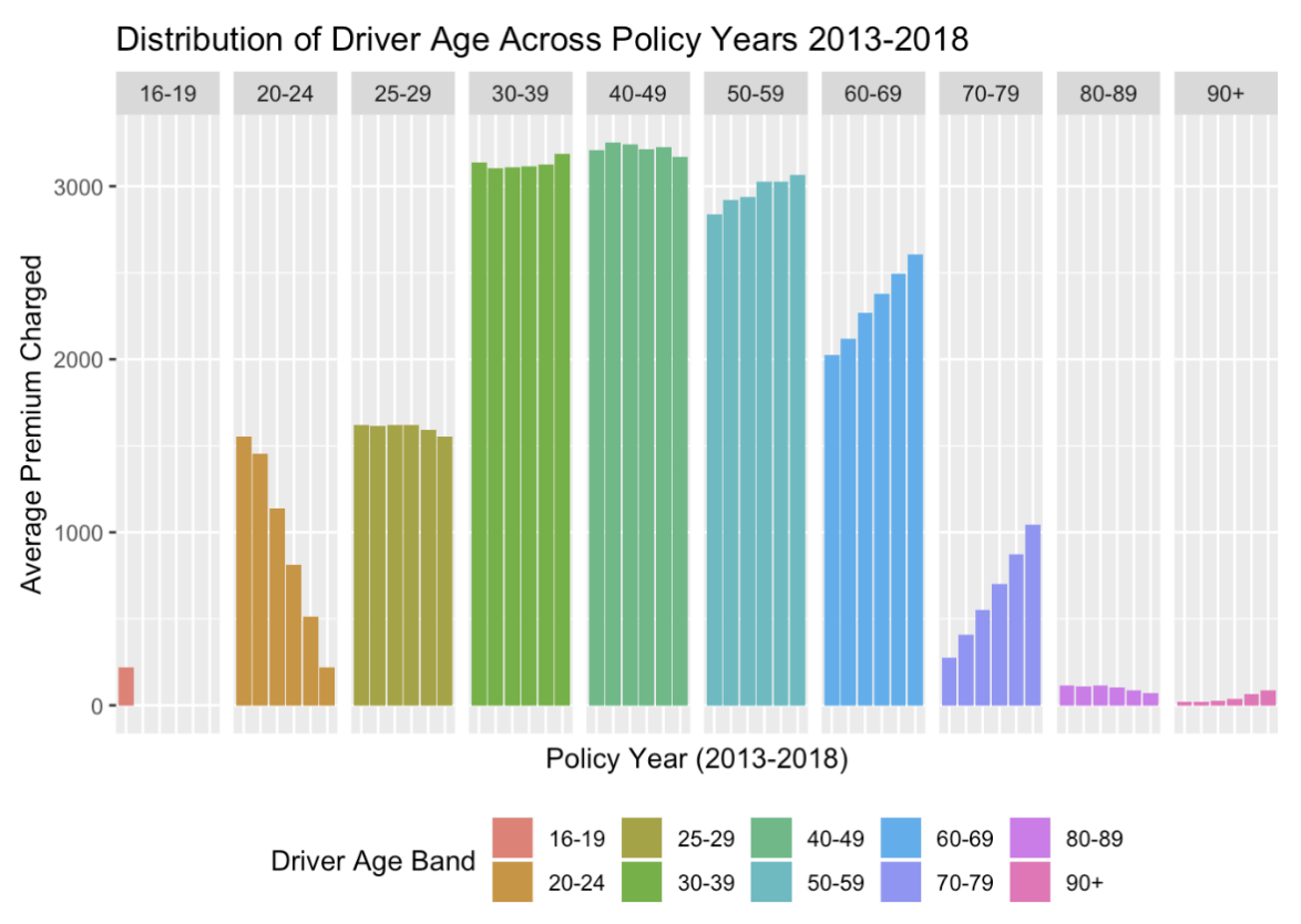
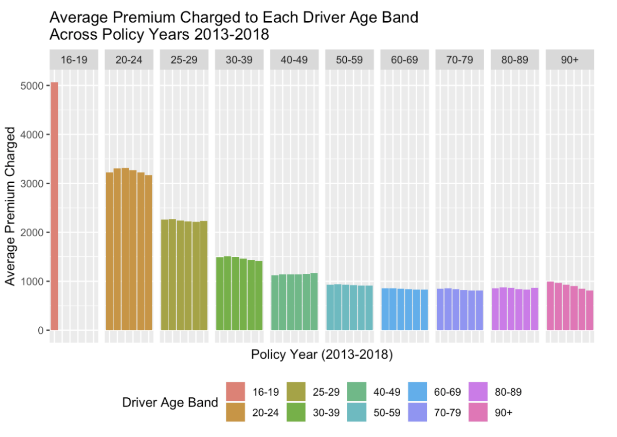
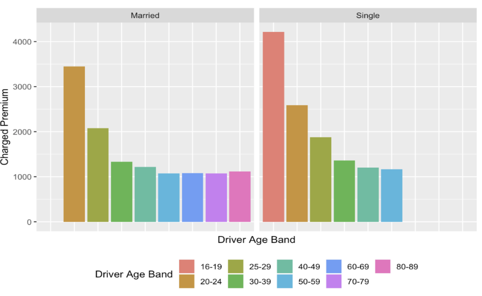
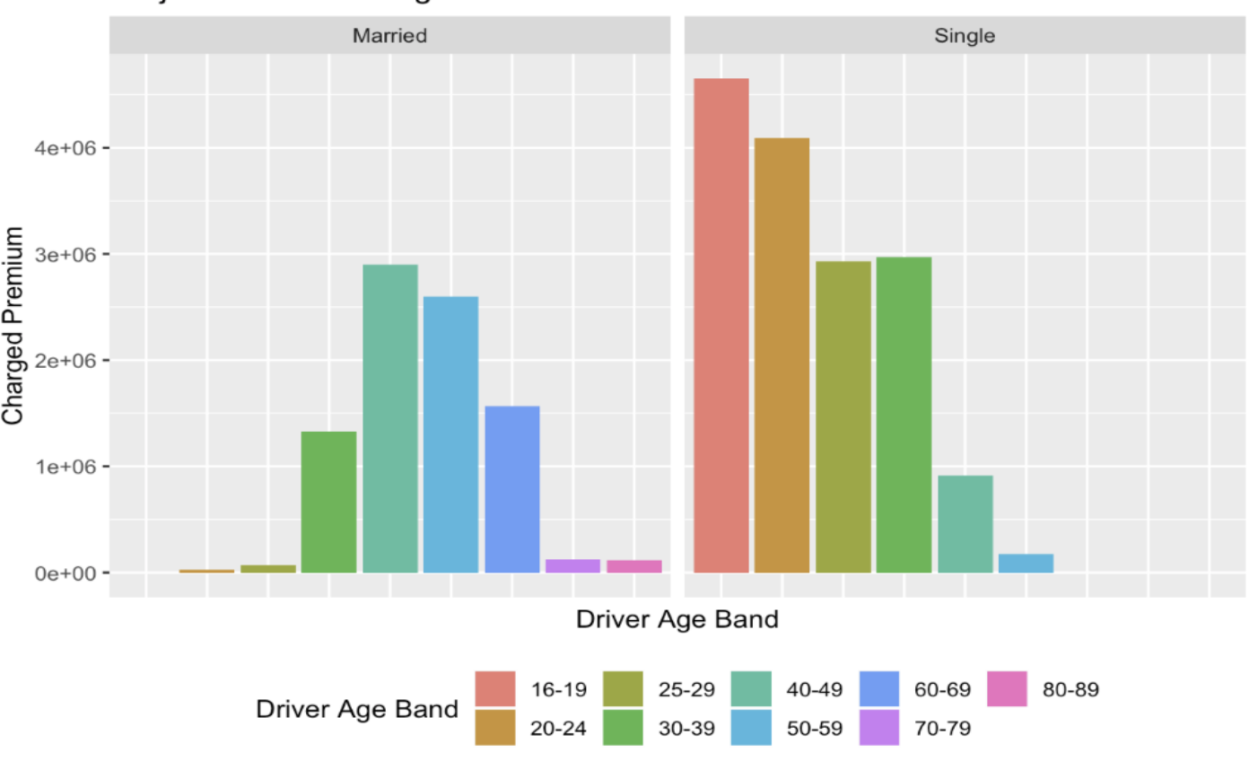
With the given data, we arrive with a number of observations and considerations. Because our private passenger automobile insurance policies are rated to a vehicle’s primary driver, we take the simplifying assumption that each vehicle has one unique primary driver at any Figure 1. Progression of age-structure of insureds in provided dataset for policy years 2013-2018. Figure 2. Progression of average charged premium over policy years 2013-2018, separated by age band. Average premiums generally decline each year. given point in time as specified in the database. Additionally, we price coverage of each vehicle separately, where it is simple to combine these per policy.
Observations: In data validation, we make a number of key observations regarding the 15,000 policyholder records in the database, for each of the policy years 2010 through 2018:
1. 33% of vehicles are part of a multi-car policy
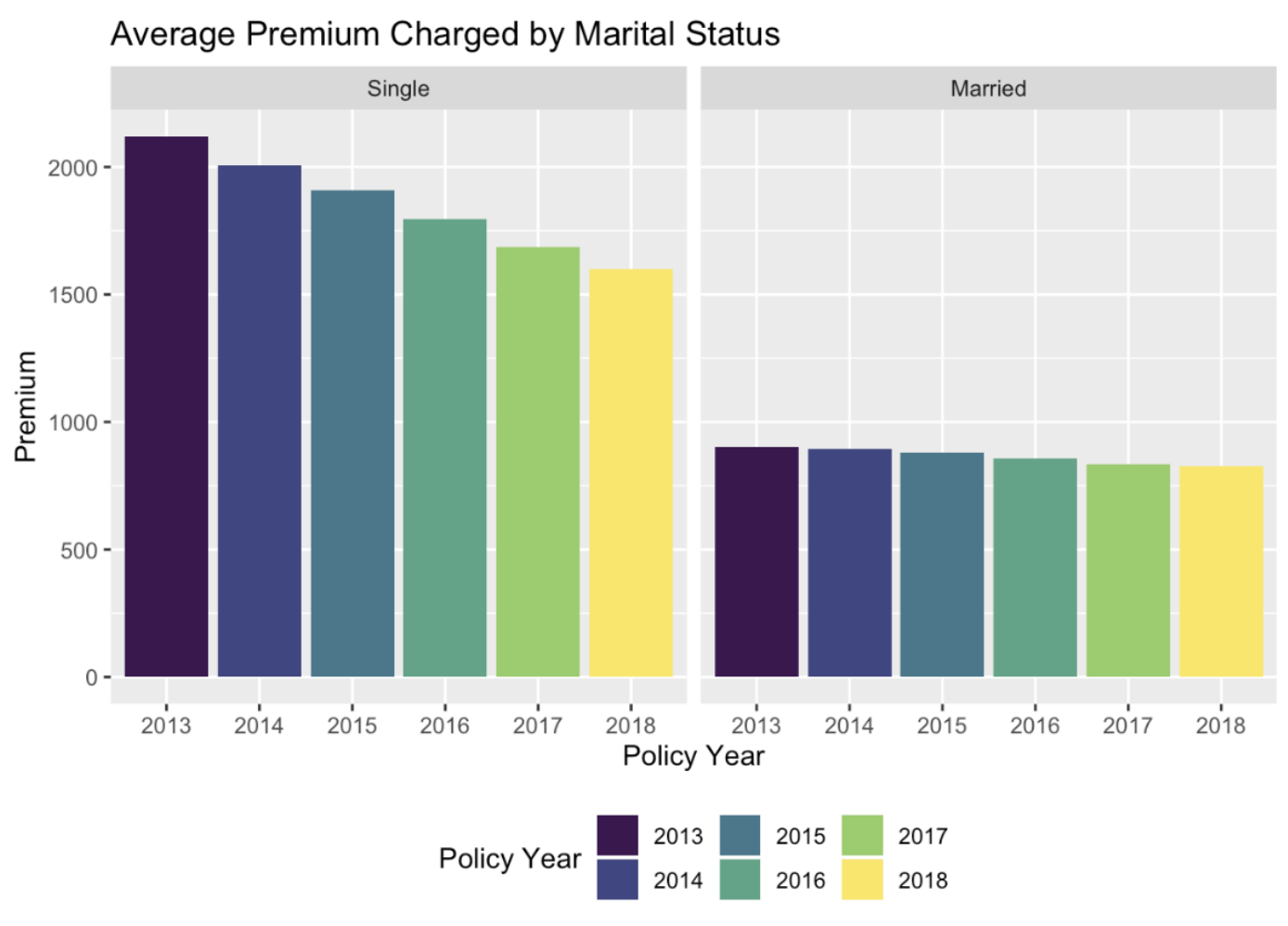
2. Roughly 50% of policyholders are single and 50% are married
3. 100% of policyholders have the same marital status, annual mileage, territory, credit score, car value, and deductible and liability limits for the entirety of the nine-year experience period
4. 100% of policyholders have zero late fees for policy years 2014, 2015, 2016, 2017, 2018
5. 100% of policyholders have zero conviction points for policy years 2016, 2017, and 2018
If this set of 15,000 individuals is a representative (random) sample of the entire population of drivers insured by Cal Insurance over these experience years, it is anomalous that all of 15,000 individuals do not move territories, change cars, adjust policy deductibles and liability limits, among other possible changes. Observations (3), (4) and (5) provide irrefutable evidence for a grave computer error or inadequate record keeping on behalf of our carriers. We advise that Cal Insurance management verify that our carriers always keep the most recent information about its insureds. Although ratemaking is prospective, a rating algorithm relies on correct classification of risk via historical experience data. The effects of the computer error and inadequate relativities are evident in the following figures.
Loss Model & Considerations:
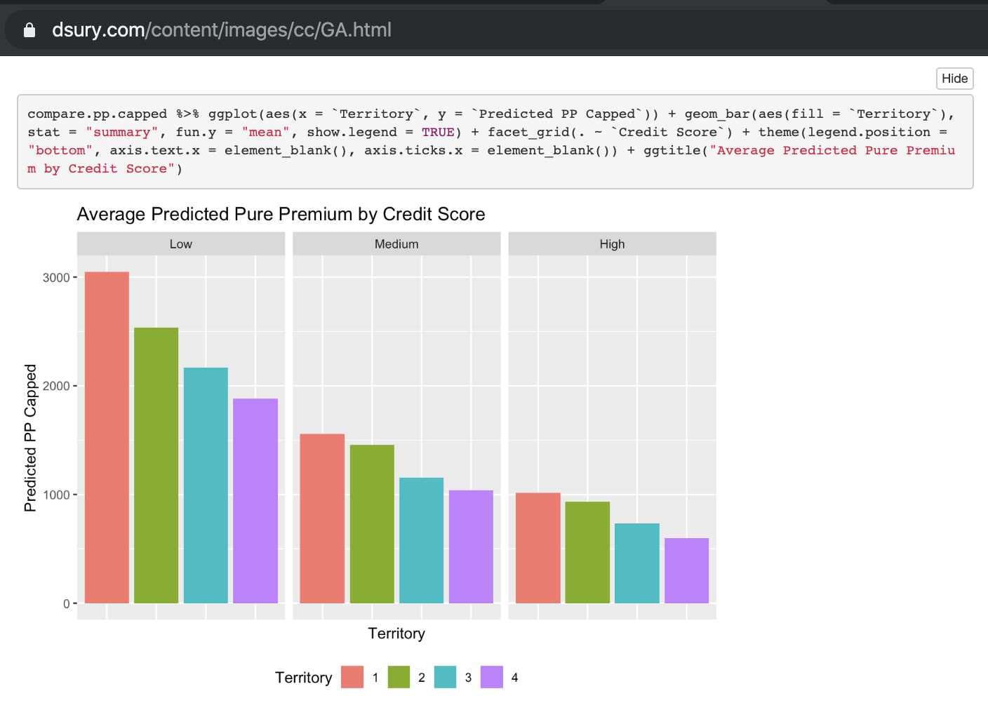
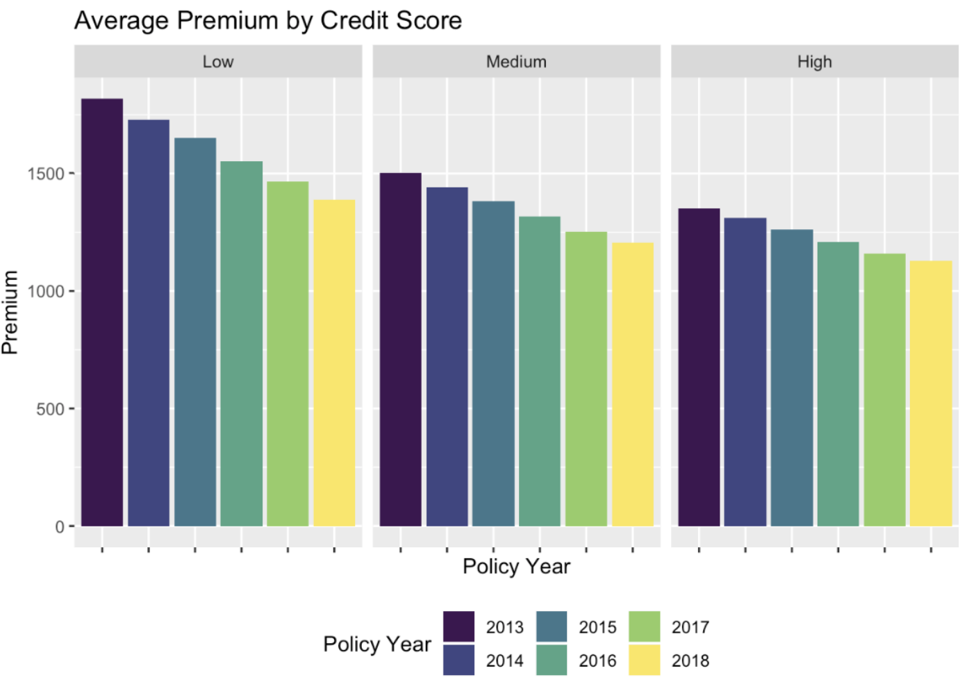
We choose the Generalized Linear Model for clarity and transparency over other machine learning methods like gradient boost, neural networks. As California requires that such rating be done via sequential analysis (minimum bias procedure), we produce our GLM for internal use only, simply as a consideration to help derive rates and underwriting algorithms Cal Insurance will file in the future. Details of assumptions and considerations from not using Credit Score to the mandated Good Driver Discount in compliance with California’s Proposition 103 are included for reference in the project documentation (interestingly, there is a clear trend in charged premium with respect to credit score, although we do not use credit score as a pricing factor). To help align with the three rating factors mandated in California, we train our GLM to (1) Driver safety record (Conviction Points), (2) Annual Mileage, and (3) Years licensed (Driving Experience) as opposed to driver’s age.
To translate from driver age to driving experience, we make the assumption that all drivers begin at age 16. Because it is commonly known to actuaries that these three mandated factors fail to adequately classify risk, we also consider (4) Accident Points and (5) Marital Status.
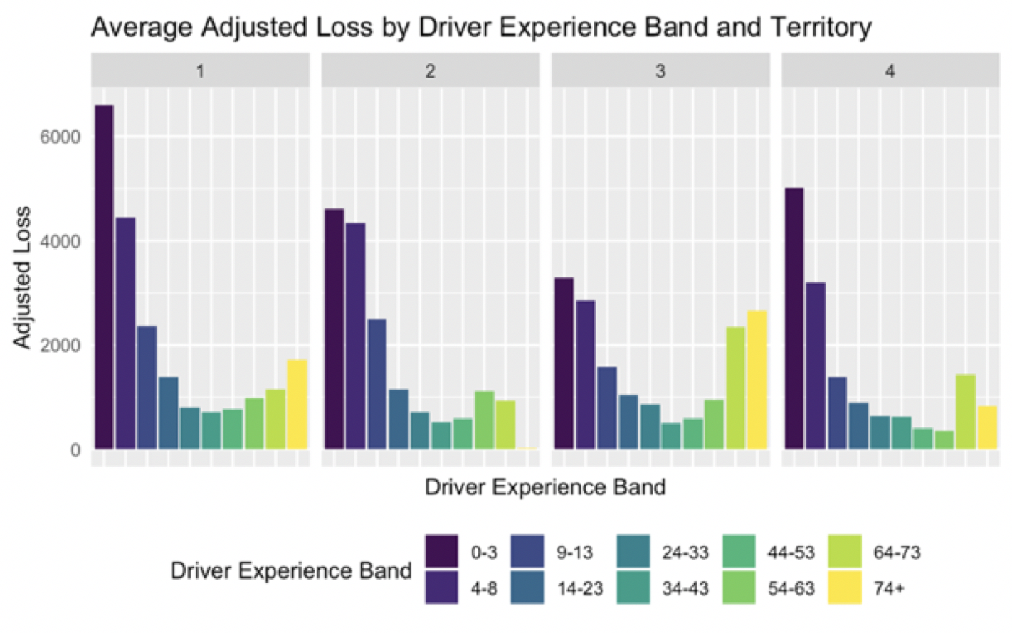
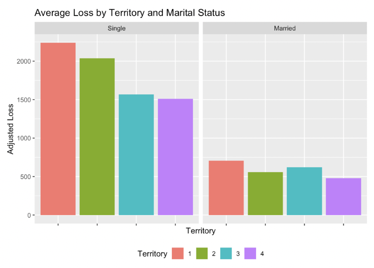
Losses across the territories are roughly monotonic as seen in Figure 6, so we include (6) Territory as a variable in our GLM as opposed to incorporating the regional factor as on offset.
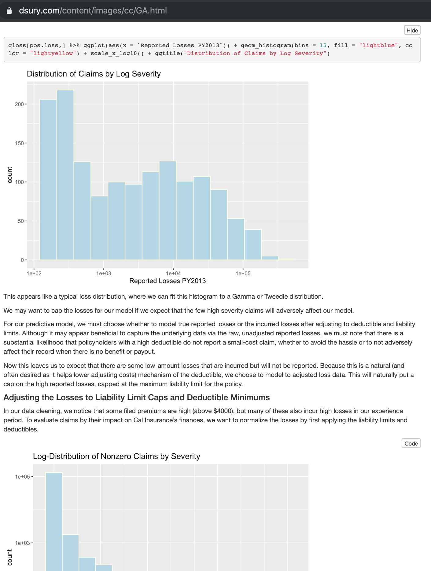
We have experimented with modeling frequency via Poisson (and negative binomial) and severity via Gamma; however, we should not assume that frequency and severity are independent. We notice 33% of vehicles are a part of a multi-car policy (observation 1 above), where we expect carpooling of married couples (and families) to affect frequency of claims with respect to the number of covered vehicles (i.e. fewer cars being driven per policy) and potentially increase severity of claims (i.e. higher liability from injuries). To address this, we directly model the pure premium as our response variable with a Tweedie distribution with power p = 1.79, which we calculated by starting with a Gamma fitted GLM to the observed severity as an estimate and iterating to maximize the log-likelihood.
Because we use Conviction Points (last 3 years) as a factor in our filed rating algorithm, we train our GLM on the only credible experience years: 2013 through 2015. As private passenger automobile is relatively a short-tailed line of business, we assume that by 2019 the paid losses in the system have developed to ultimate. For modeling, we assume that the Pure Premium is 120% of the paid loss, to account for profit load and other loss-related expenses, where such costs are assumed to scale with loss via investigation and cost containment (attorney) fees.
Model Interpretations and Business Insights:
As mentioned in our solution to Problem 2, we reject all 15,000 applicants from 2019 and require that all current and prospective insureds update their driving safety record for the past 3 years (conviction points and accident points) and submit proper documentation. This minimizes administrative costs and allows Cal Insurance to write to a broader audience. We strongly suggest this approach to compensate for the lack of credible data while upholding Cal Insurance’s trustworthy brand. Derivations of these guidelines are included in the HTML.
Underwriting Guidelines: Reject if one of the following lines applies:
1. 45+ Years Driver Experience; Single
2. 35+ Years Driver Experience; Single; 0-7500 or 10000-15000 Annual Mileage
3. <10 Years Driver Experience; Married; 0-7500 Annual Mileage
4. <15 Years Driver Experience; Married; Territory 4
5. 2+ Accident Points (last 3 years)
6. 3+ Conviction Points (last 3 years)
To generate the decisions.csv file, we trend the new application data to the same error of our current database. That is, we assume that conviction points in 2019 are accurate and insert zeroes for accident and conviction points for policy years 2017 and 2018. This provides us with a conservative estimate of premiums as shown above and we can generally expect higher premiums.
Prompt: Property & Casualty
You are the actuary for a P&C company specializing in insurance for restaurants in the state of Notliable. Due to regulation in the state of Notliable, all liability losses are covered by the state. Thus, only property losses are covered by your company. You are asked to produce a rate level indication for a January 1, 2019 rate change.
You are given:
- All policies are annual.
- Exposures are defined as “policy years.”
- Proposed effective date for the rate change is 1/1/2019.
- Rates will be in effect for one year.
- There was a 5% rate change effective January 1, 2015.
- There was a 5% rate change effective January 1, 2016.
- There was a 3% rate change effective January 1, 2017.
- There was a 6% rate change effective January 1, 2018.
- Commissions = 10.0%.
- Taxes = 3.0%.
- Variable portion of General and Other Acquisition = 4.0%.
- Profit load = 2.0%.
- Total fixed expense = 40 dollars per exposure.
- Assume no catastrophes.
Tasks:
Task 1.
What is a rate level indication? Why is it necessary?
Task 2.
On-level all premium using the parallelogram method and select a premium trend using internal data. Justify your choice.
Task 3.
a) Determine whether you will develop losses and ALAE separately or together. Justify your choice. In general, when does combining losses and ALAE make more sense? When does it not?
b) Develop reported losses and ALAE using whatever method you like. Also, please highlight any major assumptions or alterations made to the data.
c) Explain the difference between ULAE and ALAE.
Task 4
Select a loss trend using internal data. How does this loss trend compare to those offered by ISO? What is one potential weakness of the internal data?
Task 5
Trend your developed losses using either an internal or external trend. Justify your choice. Please clearly show the dates you are using to trend.
Task 6
Produce a Variable Permissible loss and ALAE ratio from the given expenses. Show the formula used.
Task 7
Using the loss ratio method and your work from tasks 1-6, what is the indicated rate level change and what does it mean for the company? Given the current indication, do previous rate changes make sense? What is the difference between the loss ratio method and pure premium method, and when might one be better than the other?
Report: Property & Casualty - Restaurant Insurance Coverage
Abstract:
As actuaries within P&C specializing in insuring restaurants, we are tasked with producing a rate level indication for a January 1, 2019 rate change. We on-level earned premiums using the traditional parallelogram method. Because the representative data are relatively thin and recent, we use a Bayesian Markov Chain Monte Carlo (MCMC) approach to develop losses and ALAE.
On-Leveling Premiums:
As an insurance company, we must calculate and estimate how much to charge for different lines and levels of coverage. In planning for the future, to hit a specified pricing target like target loss ratio, we use historical data to model future trends. To do so, we use a rate level indication, which measures the adequacy of current rates in funding historical losses. As ratemaking is prospective, we model and estimate future claims and want to ensure that the upcoming proposed effective rate change is adequate to pay for the future claims covered by the policy as well as pay for related expenses. However, in order to make this comparison of current rates to historical losses, we need to first on-level premiums, which is to bring historical premiums to the current rates.
In order to produce the rate level change, we must estimate the future loss ratio at current rates and compare this value with the permissible loss ratio. We will indicate the need for a rate increase if the expected future loss ratio is higher than the permissible loss ratio, and we will indicate a rate decrease if the expected future loss ratio is lower than the permissible loss ratio.
The parallelogram for premium adjustment does not require specific details of the underlying underwriting procedure as it assumes a uniform distribution (constant rate) of policies written throughout the year (and hence throughout the policy period). We note that rate changes can be in either direction; however, we assume that the rate changes on January 1 of the years 2015 through 2018 are all increases. Because our coverage plans are purely property-related, we reason that the historical rate changes rates may track well with inflation rate and property value, and hence indicated rate changes may be typically positive in this line of property insurance.
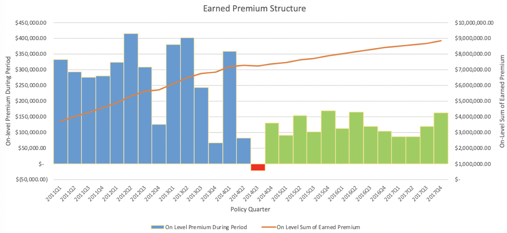
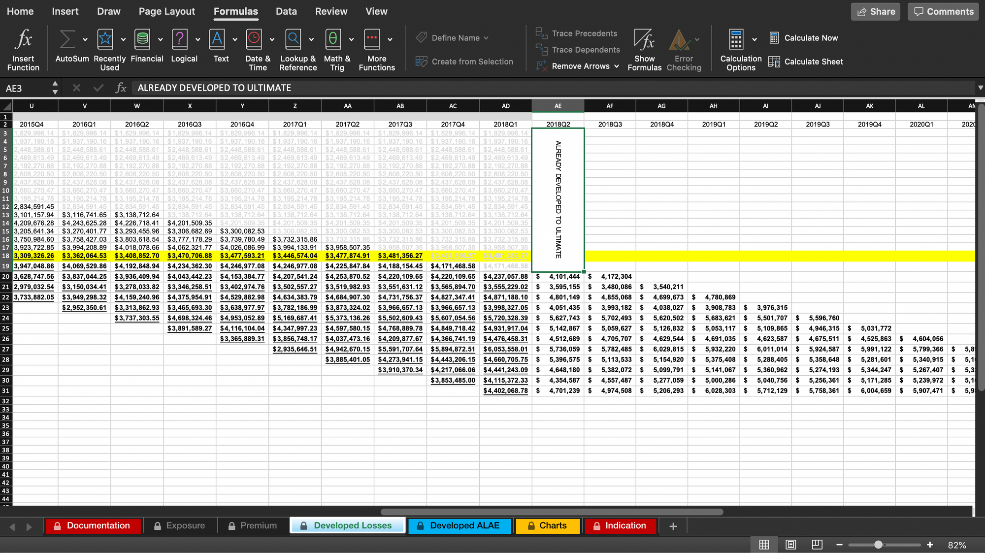
We do not expect the parallelogram method to yield a perfect result, especially with a large uncertainty in the possibility of an update in the company’s claims process. In particular, looking at unadjusted earned premium during period, we see that starting Policy Quarter 4 of year 2014, earned premiums are roughly between a third and a half of their previous values. There is high variability in the periods before, where in 2014 Quarter 3, there is even a negative earned premium during the quarter. Recall the following accounting equation for earned premium:
EP = WP + UEPR begin – UEPR end ,
where UEPR is the Unearned Premium Reserve, EP is the Earned Premium, and WP is the written premium. Because the total amount of earned pure premium during the life of a year-long policy is equal to the pure premium at the start of the policy term, the negative earned premium during 2014Q3 indicates a balance via “over-earning” either in a prior or later period. Viewing the trend in the figure above, there is strong reason to believe that that the over-earning of premium was prior to 2014Q3. As there is a substantial material change in the premium structure (as well as the exposure structure shown later below), it is possible that the assumptions made for the parallelogram method are violated.
Loss and ALAE Development:
Insurance claims incur losses to the insurer not only in the form of payouts to the policyholder but also loss-related expenses (LAE) such as legal or defense costs, salaries of insurance claims adjusters, typical business overhead costs, or even police investigation fees. In general, we may expect these payments to have schedules of their own, independent or not closely related with the rhythm of claims reporting and processing. For example, typical overhead costs such as building costs and salaries are on a regular schedule; however, an insurer specializing in P&C insurance for restaurants may experience a seasonally higher frequency of claims closer to national holidays, where restaurants might be busier.
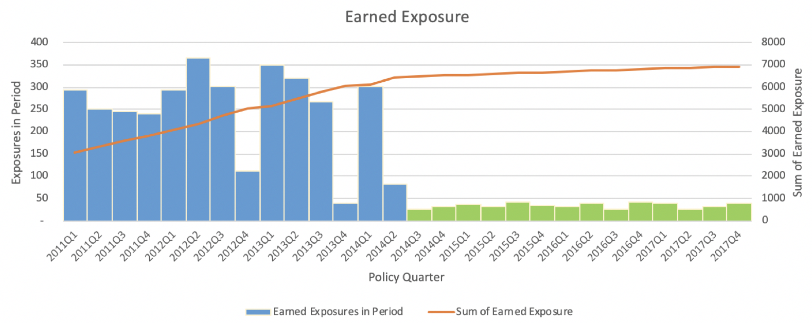
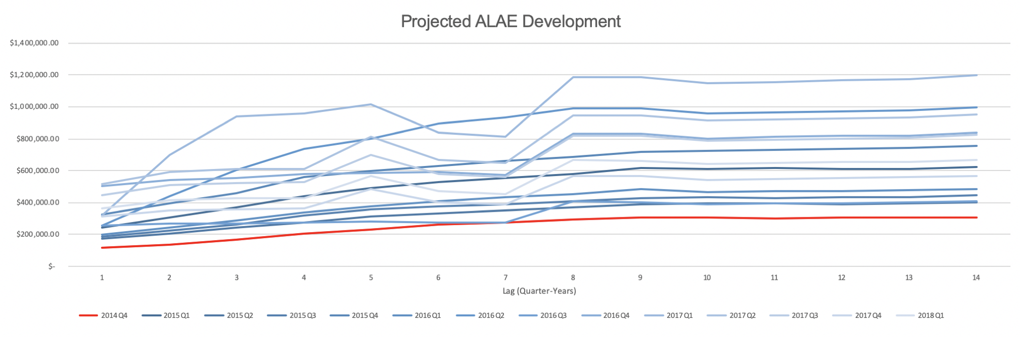
Noting the possibly large difference in schedules, we develop losses and ALAE separately, generally expecting ALAE to track the trend of loss development but with added lag as adjusters process claims. The standard loss development (Chain Ladder) technique assumes that the relative change in a given policy term’s loss from one lag period to the next is indicative of the relative change in prior experience period’s losses at the corresponding lag periods. In Figure 2 below (as well as Figure 1 reflecting the premium structure), we see that a large change in earned exposure trend. We take the region indicated in green (policy quarter 2014Q3 and after) to be representative of the current exposure trend.
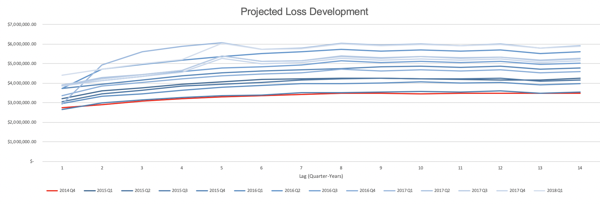
The traditional approach to loss development in cases like these is to use the Bornhuetter Ferguson method, or slightly better, the iterative adaptation. The advantages here are that random fluctuations in early experience periods do not significantly distort projections, and these methods can be used even if there are only thin or volatile data. However, due to the lack of credible data, these methods are rather reliant on the actuary’s judgement. We choose to not pursue these traditional methods because although they have their strengths, they are not responsive to underlying loss development patterns. Moreover, we certainly do not want to rely heavily on ISO data, as restaurants’ levels of risk vary greatly in terms of many factors, including geographical region, size, cooking process, and type of cuisine.
Instead, we use a Metropolis-Hastings algorithm to construct a Markov Chain Monte Carlo simulation. With recent developments in stochastic loss reserving, this Bayesian approach is empirically shown to be statistically more powerful and is well worth not only mention but also pursuit.
Rate Indication:
In excel, we’ve estimated the historical Variable Permissible Loss Ratio is 91%, the ALAE ratio is 16%, and the loss ratio is 129%. This is an indication for a rate increase to get closer to our desired margins. Using formula (1) in the appendix, we’ve calculated the indicated average premium per exposure in 2019 to be $173,666.02. This uses the Pure Premium method of overall indication. A major benefit of this approach is that it does not require on-level earned premium data to compute. However, this requires a rigorous and well-defined exposure base as we have in our case as 1 policy year. On the other hand, the Loss Ratio method is more commonly used and theoretically gives the same result. A benefit of this is to look at the overall indicated rate change, as this helps with dislocation analysis. Because this method requires on-level earned premiums, which we do not have, we simply note that the Pure Premium method yields the same result.
Raising the rates for coverage is a difficult consideration because it is needed for adequacy to pay out claims; however, this may lead to a net revenue loss if a substantial amount of policyholders cancel their insurance plans or switch to a competitor. With the necessity in mind of raising rates, the historical rate increases are in the correct direction.
Acknowledgements:
General Analytics:
Tweedie, M. C. K. (1984). An index which distinguishes between some important exponential families. In Statistics: Applications and New Directions. Proceedings of the Indian Statistical Institute Golden Jubilee International Conference. (Eds. J. K. Ghosh and J. Roy), pp. 579-604. Calcutta: Indian Statistical Institute.
Jørgensen B (1987). “Exponential Dispersion Models (with discussion).” Journal of the Royal Statistical Society, Series B, 49, 127–162.
Jee, B. (1989). A Comparative Analysis of Alternative Pure Premium Models in the Automobile Risk Classification System. The Journal of Risk and Insurance, 56(3), 434-459. doi:10.2307/253167
Nissan, Edward and Hamwi, Iskandar S., "Predicting Automobile Insurance Multi-Regional Base Pure Premiums" (1994). Journal of Actuarial Practice 1993-2006. 157. http://digitalcommons.unl.edu/joap/157
Smyth G, Jørgensen B (2002). “Fitting Tweedie’s Compound Poisson Model to Insurance Claims Data: Dispersion Modelling.” ASTIN Bulletin, 32, 143–157.
Meyers, G (2009). “Pure Premium Regression with the Tweedie Model”
https://www.casact.org/newsletter/ pdfupload/ar/brainstorms_ corrected_from_ar_may2009.pdf
Dunn PK (2011). tweedie: Tweedie Exponential Family Models. R package version 2.1.1, http: //cran.r-project.org/web/packages/tweedie
Zhang, Y (2013). Likelihood-based and Bayesian Methods for Tweedie Compound Poisson Linear Mixed Models, Statistics and Computing, 23, 743-757. https://github.com/actuaryzhang /cplm/files/144051/TweediePaper.pdf
Property & Casualty:
Metropolis, N., S. Ulam. (1949). “The Monte Carlo Method.” Journal of the American Statistical Association 44(247):335–341.
Hastings, W. K. (1970). “Monte Carlo Sampling Methods Using Markov Chains and Their Applications.” Biometrika 57(1):97–109.
Bornhuetter, R.L., Ferguson R.E. (1972). “The Actuary and IBNR.” Proceedings of the Casualty Actuarial Society 59:181–195.
Almagro, M.; Ghezzi, T.L. (1988). “Federal Income Taxes --- Provisions Affecting Property/Casualty Insurers,” PCAS LXXV.
Gelfand, A. E., Smith A.F.M. (1990). “Sampling-Based Approaches to Calculating Marginal Densities.” Journal of the American Statistical Association 85(410): 398–409.
Insurance Accounting and Systems Association (1994). Property-Casualty Insurance Accounting (6th Ed)
Bowers, N.L.; Gerber, H.U.; Hickman, J.C.; Jones, D.A.; Nesbit, C.J (1997). Actuarial Mathematics (2nd Ed)
Werner, G.; Modlin, C. (2010). Basic Ratemaking. 2nd ed. Casualty Actuarial Society
Klugman, S.A., Panjer, H.H, Willmot, G.E. (2012). Loss Models, From Data to Decisions, 4th edition. Hoboken, NJ: Wiley
Zhang Y. (2010). A general multivariate chain ladder model. Insurance: Mathematics and Economics, 46, pp. 588:599.